본문으로 건너뛰기

절1.2행 축약

목표
  1. 연립일차방정식을 첨가행렬로 바꾸어 나타내는 방법을 배웁니다.
  2. 소거법이 첨가행렬에 행 연산을 수행하는 것과 어떻게 대응하는지 배웁니다.
  3. 행렬이 언제 (기약) 행 사다리꼴인지 이해합니다.
  4. 행 축약된 행렬 중 어떤 것이 불능인 연립일차방정식에서 나오는지 알아봅니다.
  5. 계산 절차: 행 축약 알고리즘.
  6. 용어: 행 연산, 행 동치, 행렬, 첨가행렬, 피벗, (기약) 행 사다리꼴.

이 절에서는 연립일차방정식을 “푸는” 알고리즘을 제시합니다.

소절1.2.1소거법

우리는 소거법을 사용하여 연립일차방정식을 대수적으로 풀 것입니다. 다시 말해, 방정식들을 여러 방식으로 결합하여 각 방정식에서 가능한 한 많은 변수를 소거하려고 합니다. 연립방정식에 수행할 수 있는 유효한 연산은 세 가지입니다.


  • 스케일링: 방정식의 양변에 0이 아닌 수를 곱할 수 있습니다.
    \begin{equation*}
\syseq{x + 2y + 3z = 6;
2x - 3y + 2z = 14;
3x + y - z = -2
} \quad\xrightarrow{\text{multiply 1st by $-3$}}\quad
\syseq{-3x - 6y - 9z = -18;
2x - 3y + 2z = 14;
3x + y - z = -2
}
\end{equation*}
  • 치환: 한 방정식의 배수를 다른 방정식에 더하고, 그 결과로 두 번째 방정식을 대체할 수 있습니다.
    \begin{equation*}
\syseq{x + 2y + 3z = 6;
2x - 3y + 2z = 14;
3x + y - z = -2
} \quad\xrightarrow{\text{2nd ${}={}$ 2nd$-2\times$1st}}\quad
\syseq{x + 2y + 3z = 6;
\. \+ -7y - 4z = 2;
3x + y - z = -2
}
\end{equation*}
  • 교환: 두 방정식의 위치를 바꿀 수 있습니다.
    \begin{equation*}
\syseq{x + 2y + 3z = 6;
2x - 3y + 2z = 14;
3x + y - z = -2
} \quad\xrightarrow{\text{3rd $\longleftrightarrow$ 1st}}\quad
\syseq{3x + y - z = -2;
2x - 3y + 2z = 14;
x + 2y + 3z = 6
}
\end{equation*}
첨가행렬과 행 연산

소거법으로 방정식을 풀려면 단지 자리 표시를 위해 변수 x,y,z와 등호 =를 계속해서 반복하여 써야 합니다. 방정식에서 실제로 바뀌는 것은 계수인 수뿐입니다. 숫자만 뽑아내어 상자에 넣으면, 즉 첨가행렬로 나타내면 일이 훨씬 수월해집니다:

\begin{equation*}
\syseq{x + 2y + 3z = 6;
2x - 3y + 2z = 14;
3x + y - z = -2
}
\quad\xrightarrow{\text{becomes}}\quad
\amat{
1  2  3  6 ;
2  -3  2  14;
3  1  -1  -2
}.
\end{equation*}

이것을 첨가행렬이라고 합니다. “첨가”라는 말은 등호가 어디에 있는지 상기하기 위해 그리는 세로선을 가리킵니다. 행렬은 세로선이 없는 수의 격자입니다. 이 표기법에서 방정식을 다루는 세 가지 유효한 방법은 행 연산이 됩니다.

  • 스케일링: 한 행의 모든 성분에 0이 아닌 수를 곱합니다.
    \begin{equation*}
\amat{
1  2  3  6 ;
2  -3  2  14;
3  1  -1  -2
}
\quad\xrightarrow{R_1 = R_1 \times -3}\quad
\amat{
-3  -6  -9  -18 ;
2  -3  2  14;
3  1  -1  -2
}
\end{equation*}
    여기서 행 연산에 쓰인 R_1이라는 표기는 단순히 “첫 번째 행”을 뜻하며, R_2,R_3, 등도 마찬가지입니다.
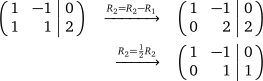
  • 대체: 한 행에 다른 행의 상수배를 더하고, 두 번째 행을 그 결과로 대체하는 행 연산입니다.
    \begin{equation*}
\amat{
1  2  3  6 ;
2  -3  2  14;
3  1  -1  -2
}
\quad\xrightarrow{R_2 = R_2 -2\times R_1}\quad
\amat{
1  2  3  6 ;
0 -7 -4 2;
3  1  -1  -2
}
\end{equation*}
  • 교환: 두 행을 서로 맞바꾸는 행 연산입니다.
    \begin{equation*}
\amat{
1  2  3  6 ;
2  -3  2  14;
3  1  -1  -2
}
\quad\xrightarrow{R_1 \longleftrightarrow R_3}\quad
\amat{
3  1  -1  -2;
2  -3  2  14;
1  2  3  6
}
\end{equation*}

행렬에 행 연산을 하는 과정은 대응하는 일차방정식들의 해집합을 바꾸지 않습니다!

사실 이러한 연산을 하는 목적은 바로 소거법을 사용하여 방정식을 푸는 데 있습니다.

정의

두 행렬 중 하나에 행 연산을 몇 번 하여 다른 하나를 얻을 수 있으면 두 행렬을 행 동치라고 합니다.

따라서 행 동치인 행렬들의 일차방정식은 같은 해집합을 가집니다.

소절1.2.2사다리꼴

앞 소절에서 연립일차방정식을 첨가행렬로 옮기는 방법을 살펴보았습니다. 이제 그러한 첨가행렬을 “푸는” 알고리즘을 찾고자 합니다. 먼저 첨가행렬이 “풀렸다”는 것이 무엇을 뜻하는지 정해야 합니다.

정의

다음 조건을 만족하는 행렬은 행 사다리꼴입니다:

  1. 모든 영행은 맨 아래에 있습니다.
  2. 각 행의 0이 아닌 첫 성분은 바로 위 행의 0이 아닌 첫 성분보다 오른쪽에 있습니다.
  3. 한 행의 0이 아닌 첫 성분 아래에 있는 성분은 모두 0입니다.

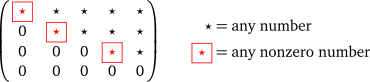
다음은 행 사다리꼴 행렬을 그림으로 나타낸 것입니다:

\begin{equation*}
\mat{
\color{red}\boxed\star,  \star,  \star,  \star,  \star ;
0  \color{red}\boxed\star,  \star,  \star,  \star ;
0  0  0  \color{red}\boxed\star, \star ;
0 0 0 0 0}\qquad
\begin{aligned}
\star &= \text{any number} \\
\color{red}\boxed\star &= \text{any nonzero number}
\end{aligned}
\end{equation*}
정의

피벗은 행 사다리꼴 행렬에서 각 행의 0이 아닌 첫 성분입니다.

행 사다리꼴 행렬은 일반적으로 후진 대입을 사용하여 쉽게 풀 수 있습니다. 예를 들어,

\begin{equation*}
\amat{
1  2  3  6 ;
0 1 2 4 ;
0 0 10 30
} \quad\xrightarrow{\text{becomes}}\quad
\syseq{
x + 2y + 3z = 6;
\. \+ y + 2z = 4;
\. \+ \. \+ 10z = 30\rlap.}
\end{equation*}

바로 z=3임을 알 수 있으며, 이로부터 y = 4-2\cdot 3 = -2이고 x = 6 - 2(-2) - 3\cdot 3 = 1.임을 얻습니다. 이 예제을 참고하십시오.

정의

행렬이 행 사다리꼴이면서 다음 조건을 추가로 만족하면 그 행렬은 기약 행 사다리꼴입니다:

  1. 각 피벗은 1입니다.
  2. 각 피벗은 그 열에서 유일한 0이 아닌 성분입니다.

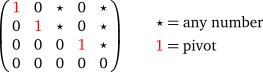
다음은 기약 행 사다리꼴 행렬을 그림으로 나타낸 것입니다:

\begin{equation*}
\mat{
\color{red}1   0   \star,   0   \star ;
0   \color{red}1   \star , 0   \star ;
0   0   0   \color{red}1   \star ;
0 0 0 0 0
} \qquad
\begin{aligned}
\star &= \text{any number} \\
\color{red}1 &= \text{pivot}
\end{aligned}
\end{equation*}

기약 행 사다리꼴 행렬은 어떤 의미에서 완전히 풀린 상태입니다. 예를 들어,
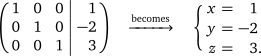
\begin{equation*}
\amat{
1  0 0 1 ;
0 1 0 -2 ;
0 0 1 3
} \quad\xrightarrow{\text{becomes}}\quad
\syseq{
x = 1; y = -2; z = 3\rlap.}
\end{equation*}

첨가행렬이 (기약) 행 사다리꼴인지 판단할 때, 첨가된 열을 특별하게 취급할 필요는 없습니다. 세로선은 그냥 무시하십시오.

첨가행렬이 기약 행 사다리꼴이면, 대응하는 연립일차방정식은 풀린 것으로 간주합니다. 왜 그런지는 아래에서 살펴볼 것이며, 어떤 행렬이든 행 연산만으로 기약 행 사다리꼴로 만들 수 있음을 보일 것입니다.

소절1.2.3행 축약 알고리즘

모든 행렬이 적어도 하나의 기약 행 사다리꼴 행렬과 행 동치임을 보여 주는 알고리즘을 제시할 것이며, 이를 행 축약 또는 가우스 소거법이라고 합니다.

유일성에 관한 명제는 흥미롭습니다—이 명제는 어떤 방식으로 행 축약을 하든 항상 같은 기약 행 사다리꼴 행렬을 얻는다는 뜻입니다.

물론 이는 허용된 세 가지 행 연산만 수행하고 계산 실수를 하지’ 않는다는 것을 전제로 합니다.

유일성을 증명하지는 않겠지만, 여러분은 증명할 수 있을지도 모릅니다!

다음은 행렬의 행 축약 알고리즘을 그림으로 요약한 것입니다.
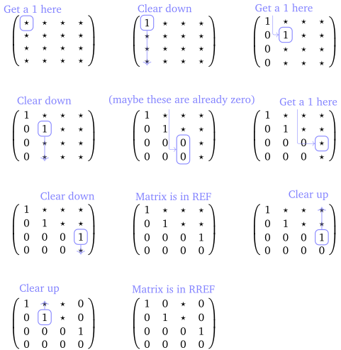
\begin{tikzpicture}
  \tikzset{
    my matrix/.style={
      matrix, math matrix, anchor=west, row sep=.5em,
          every node/.append style={minimum width=1em, minimum height=.666em}},
    blue box/.style={
      draw,thick,rounded corners,blue!50,fit=#1,inner xsep=1pt}
  };

  \path node[my matrix] (m1) {
    \star \& \star \& \star \& \star \\
    \star \& \star \& \star \& \star \\
    \star \& \star \& \star \& \star \\
    \star \& \star \& \star \& \star \\
  } (m1.west) ++(4.5cm,0) node[my matrix] (m2) {
    1 \& \star \& \star \& \star \\
    \star \& \star \& \star \& \star \\
    \star \& \star \& \star \& \star \\
    \star \& \star \& \star \& \star \\
  } (m2.west) ++(4.5cm,0) node[my matrix] (m3) {
    1 \& \star \& \star \& \star \\
    0 \& 1 \& \star \& \star \\
    0 \& \star \& \star \& \star \\
    0 \& \star \& \star \& \star \\
  } (m1.west) ++(0,-3.5cm) node[my matrix] (m4) {
    1 \& \star \& \star \& \star \\
    0 \& 1 \& \star \& \star \\
    0 \& \star \& \star \& \star \\
    0 \& \star \& \star \& \star \\
  } (m2.west) ++(0,-3.5cm) node[my matrix] (m5) {
    1 \& \star \& \star \& \star \\
    0 \& 1 \& \star \& \star \\
    0 \& 0 \& 0 \& \star \\
    0 \& 0 \& 0 \& \star \\
  } (m3.west) ++(0,-3.5cm) node[my matrix] (m6) {
    1 \& \star \& \star \& \star \\
    0 \& 1 \& \star \& \star \\
    0 \& 0 \& 0 \& \star \\
    0 \& 0 \& 0 \& \star \\
  } (m4.west) ++(0,-3.5cm) node[my matrix] (m7) {
    1 \& \star \& \star \& \star \\
    0 \& 1 \& \star \& \star \\
    0 \& 0 \& 0 \& 1 \\
    0 \& 0 \& 0 \& \star \\
  } (m5.west) ++(0,-3.5cm) node[my matrix] (m8) {
    1 \& \star \& \star \& \star \\
    0 \& 1 \& \star \& \star \\
    0 \& 0 \& 0 \& 1 \\
    0 \& 0 \& 0 \& 0 \\
  } (m6.west) ++(0,-3.5cm) node[my matrix] (m9) {
    1 \& \star \& \star \& \star \\
    0 \& 1 \& \star \& \star \\
    0 \& 0 \& 0 \& 1 \\
    0 \& 0 \& 0 \& 0 \\
  } (m7.west) ++(0,-3.5cm) node[my matrix] (m10) {
    1 \& \star \& \star \& 0 \\
    0 \& 1 \& \star \& 0 \\
    0 \& 0 \& 0 \& 1 \\
    0 \& 0 \& 0 \& 0 \\
  } (m8.west) ++(0,-3.5cm) node[my matrix] (m11) {
    1 \& 0 \& \star \& 0 \\
    0 \& 1 \& \star \& 0 \\
    0 \& 0 \& 0 \& 1 \\
    0 \& 0 \& 0 \& 0 \\
  }
  ;

  \node [blue box=(m1-1-1)] (bm1-1-1) {};
  \node [blue!50, above=1mm of m1-1-1, anchor=south west, xshift=-1cm, align=left]
    (expl1) {Get a $1$ here};

  \node [blue box=(m2-1-1)] (bm2-1-1) {};
  \node [blue!50, above=1mm of m2-1-1, anchor=south west, xshift=-5mm, align=left]
    (expl2) {Clear down};
  \draw[->, blue!50, very thick, opacity=.5] (bm2-1-1.south) -- (m2-4-1.south);

  \node [blue box=(m3-2-2)] (bm3-2-2) {};
  \node [blue!50, above=1mm of m3-1-2, anchor=south, xshift=-.65mm, align=center]
    (expl3) {Get a $1$ here};
  \draw[->, blue!50, rounded corners=.5mm]
      (expl3.215) |- (bm3-2-2.west);

  \node [blue box=(m4-2-2)] (bm4-2-2) {};
  \node [blue!50, above=1mm of m4-1-1, anchor=south west, xshift=-5mm, align=left]
    (expl4) {Clear down};
  \draw[->, blue!50, very thick, opacity=.5] (bm4-2-2.south) -- (m4-4-2.south);

  \node [blue box=(m5-3-3) (m5-4-3)] (bm5-2) {};
  \node [blue!50, above=1mm of m5-1-3, anchor=south, xshift=-.55mm, align=center]
    (expl6) {(maybe these are already zero)};
  \draw[->, blue!50, rounded corners=.5mm]
      (expl6.215) |- (bm5-2.west);

  \node [blue box=(m6-3-4)] (bm6-3-4) {};
  \node [blue!50, above=1mm of m6-1-4, anchor=south, xshift=-5mm, align=center]
    (expl7) {Get a $1$ here};
  \draw[->, blue!50, rounded corners=.5mm]
      (expl7.215) |- (bm6-3-4.west);

  \node [blue box=(m7-3-4)] (bm7-3-4) {};
  \node [blue!50, above=1mm of m7-1-4, anchor=south, xshift=-5mm, align=left]
    (expl8) {Clear down};
  \draw[->, blue!50, very thick, opacity=.5] (bm7-3-4.south) -- (m7-4-4.south);

  \node [blue!50, above=1mm of m8-1-2.north east, anchor=south, align=center, xshift=1mm]
    (expl9) {Matrix is in REF};

  \node [blue box=(m9-3-4)] (bm9-3-4) {};
  \node [blue!50, above=1mm of m9-1-4, anchor=south, xshift=-5mm, align=left]
    (expl10) {Clear up};
  \draw[->, blue!50, very thick, opacity=.5] (bm9-3-4.north) -- (m9-1-4.north);

  \node [blue box=(m10-2-2)] (bm10-2-2) {};
  \node [blue!50, above=1mm of m10-1-2, anchor=south, xshift=-2mm, align=left]
    (expl11) {Clear up};
  \draw[->, blue!50, very thick, opacity=.5] (bm10-2-2.north) -- (m10-1-2.north);

  \node [blue!50, above=1mm of m11-1-2.north east, anchor=south, align=center, xshift=1mm]
    (expl9) {Matrix is in RREF};


  \node [blue!50, below=2cm of m9-4-2.south east, anchor=north, align=center, xshift=1mm]
    (expl9) {};

\end{tikzpicture}

행 축약 후 행렬의 피벗이 어디에 있는지 아는 것은 매우 중요합니다. 이것이 다음 용어를 도입하는 이유입니다.

정의

행렬의 피벗 위치란 그 행렬의 행 사다리꼴에서 피벗이 되는 성분입니다.

행렬의 피벗 열이란 피벗 위치를 포함하는 열입니다.

위 예제에서 불능인 연립방정식의 기약 행 사다리꼴을 알아보는 방법을 보았습니다.

다시 말해, 불능인 연립방정식의 행 축약된 행렬은 다음과 같은 모양입니다:
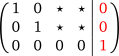
\begin{equation*}
\amat{
1  0  \star,  \star,  \color{red}0 ;
0  1  \star,  \star,  \color{red}0 ;
0  0  0  0  \color{red}1
}
\end{equation*}

지금까지 두 부류의 행렬을 다루었습니다.

  1. 행렬의 기약 행 사다리꼴이 첨가되지 않은 모든 열에 피벗을 가지면, 그 행렬은 유일한 해를 갖는 연립방정식에 대응합니다:
    \begin{equation*}
\amat{1 0 0 1; 0 1 0 -2; 0 0 1 3}
\quad\xrightarrow{\text{translates to}}\quad
\syseq{x \+ \. \+ \. = 1;
\. \+ y \+ \. = -2;
\. \+ \. \+ z = 3\rlap.}
\end{equation*}
  2. 행렬의 기약 행 사다리꼴이 마지막(첨가된) 열에 피벗을 가지면, 그 행렬은 해가 없는 연립방정식에 대응합니다:
    \begin{equation*}
\amat{1 5 0; 0 0 1}\quad\xrightarrow{\text{translates to}}\quad
\syseq{x + 5y = 0; \. \+ 0 = 1\rlap.}
\end{equation*}

첨가되지 않은 열 중 하나에 피벗이 없으면 어떻게 됩니까? 이것이 절 1.3의 주제입니다.