절4.3행렬식과 부피¶ 고유 링크

목표

행렬의 행렬식과 평행육면체의 부피 사이의 관계를 이해합니다.
행렬식을 사용하여 평행사변형과 삼각형의 부피를 계산하는 방법을 배웁니다.
행렬식을 사용하여 타원과 같은 곡선 도형의 부피를 계산하는 방법을 배웁니다.
그림: 평행육면체, 선형변환에 의한 곡선 도형의 상.
정리: 행렬식과 부피.
용어: 평행육면체.

이 절에서는 행렬식을 부피의 관점에서 기하학적으로 해석합니다. 이를 통해 행렬식의 정의 성질 네 가지 중 세 가지가 성립하는 이유를 알 수 있습니다. 또한 이는 다변수 미적분학의 변수변환 공식에서 핵심적인 요소입니다.

소절4.3.1평행사변형과 평행육면체

행렬식은 다음과 같은 기하학적 대상의 부피를 계산합니다.

정의

$\R^n$ 의 $n$ 개 벡터 $v_1, v_2,\ldots,v_n$ 이 결정하는 평행육면체는 다음 부분집합입니다.

$\begin{equation*} P = \bigl\{a_1x_1 + a_2x_2 + \cdots + a_nx_n \bigm| 0 \leq a_1,a_2,\ldots,a_n\leq 1\bigr\}. \end{equation*}$

다시 말해, 평행육면체는 계수가 $[0,1]$ 에 속하는 $n$ 개 벡터의 모든 일차결합의 집합입니다. 벡터 덧셈의 평행사변형 법칙을 이용하여 평행육면체를 그릴 수 있습니다.

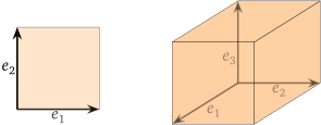
예제(단위 정육면체)

표준 좌표 벡터 $e_1,e_2,\ldots,e_n$ 이 결정하는 평행육면체는 $n$ 차원 단위 정육면체입니다.

$\begin{tikzpicture}[thin border nodes, scale=2] \filldraw[fill=seq-orange, fill opacity=.2, very thin] (0,0) -- (1,0) -- (1,1) -- (0,1) -- cycle; \draw[vector] (0,0) -- node[auto]{$e_2$} (0,1); \draw[vector, opacity=.75] (0,0) -- node[auto,swap]{$e_1$} (1,0); \end{tikzpicture} \qquad\qquad \begin{tikzpicture}[thin border nodes, myxyz, scale=2, baseline=-1cm] \def\va{(1,0,0)} \def\vb{(0,1,0)} \def\vc{(0,0,1)} \tikzmath{ coordinate \vab; coordinate \vac; coordinate \vbc; \vab = \va + \vb; \vac = \va + \vc; \vbc = \vb + \vc; } \filldraw[fill=seq-orange, opacity=.2, very thin] (0,0,0) -- \vb -- (\vbc) -- \vc -- cycle; \filldraw[fill=seq-orange, opacity=.2, very thin] (0,0,0) -- \vb -- (\vab) -- \va -- cycle; \filldraw[fill=seq-orange, opacity=.2, very thin] (0,0,0) -- \va -- (\vac) -- \vc -- cycle; \filldraw[fill=seq-orange, fill opacity=.2, shift={\vb}, very thin] (0,0,0) -- \va -- (\vac) -- \vc -- cycle; \filldraw[fill=seq-orange, fill opacity=.2, shift={\va}, very thin] (0,0,0) -- \vb -- (\vbc) -- \vc -- cycle; \filldraw[fill=seq-orange, fill opacity=.2, shift={\vc}, very thin] (0,0,0) -- \vb -- (\vab) -- \va -- cycle; \draw[vector, opacity=.4] (0,0,0) -- node[auto] {$e_1$} \va; \draw[vector, opacity=.4] (0,0,0) -- node[auto, swap] {$e_2$} \vb; \draw[vector, opacity=.4] (0,0,0) -- node[auto,pos=.3] {$e_3$} \vc; \end{tikzpicture}$

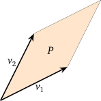
예제(평행사변형)

$n = 2$ 일 때 평행육면체는 단지 $\R^2$ 의 평행사변형입니다. 변들이 평행한 쌍을 이룬다는 점에 유의하십시오.

$\begin{tikzpicture}[thin border nodes, scale=1.3] \filldraw[fill=seq-orange, fill opacity=.2, very thin] (0,0) -- (1,2) -- (3,3) -- (2,1) -- cycle; \draw[vector] (0,0) -- node[auto]{$v_2$} (1,2); \draw[vector] (0,0) -- node[auto,swap]{$v_1$} (2,1); \node at (1.5,1.5) {$P$}; \end{tikzpicture}$

예제

$n=3$ 일 때 평행육면체는 일종의 비스듬한 정육면체입니다. 면들이 평행한 쌍을 이룬다는 점에 유의하십시오.

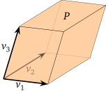
$\begin{tikzpicture}[thin border nodes, myxyz, scale=2] \filldraw[fill=seq-orange, opacity=.2, very thin] (0,0,0) -- (-1,0,0) -- (-1,.3,1) -- (0,.3,1) -- cycle; \filldraw[fill=seq-orange, opacity=.2, very thin] (0,0,0) -- (-1,0,0) -- (-.8,1,0) -- (.2,1,0) -- cycle; \filldraw[fill=seq-orange, opacity=.2, shift={(-1,0,0)}, very thin] (0,0,0) -- (.2,1,0) -- (.2,1.3,1) -- (0,.3,1) -- cycle; \filldraw[fill=seq-orange, fill opacity=.2, very thin] (0,0,0) -- (.2,1,0) -- (.2,1.3,1) -- (0,.3,1) -- cycle; \filldraw[fill=seq-orange, fill opacity=.2, shift={(.2,1,0)}, very thin] (0,0,0) -- (-1,0,0) -- (-1,.3,1) -- (0,.3,1) -- cycle; \filldraw[fill=seq-orange, fill opacity=.2, shift={(0,.3,1)}, very thin] (0,0,0) -- (-1,0,0) -- (-.8,1,0) -- (.2,1,0) -- cycle; \draw[vector] (0,0,0) -- node[auto,swap] {$v_1$} (.2,1,0); \draw[vector, opacity=.4] (0,0,0) -- node[auto,swap] {$v_2$} (-1,0,0); \draw[vector] (0,0,0) -- node[auto] {$v_3$} (0,.3,1); \node at (0,1.2,1.2) {$P$}; \end{tikzpicture}$

평행육면체의 부피가 0이 되는 것은 언제입니까? 이는 평행육면체가 납작한 경우, 즉 더 낮은 차원으로 찌그러진 경우에만 일어날 수 있습니다.

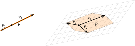
$\begin{tikzpicture}[thin border nodes, baseline=0] \draw[line width=1mm, seq-orange] (-1,-.5) to["$P$"' black] (2,1); \draw[vector, opacity=.75] (0,0) to["$v_1$" opacity=1] (2,1); \draw[vector, opacity=.75] (0,0) to["$v_2$"' opacity=1] (-1,-.5); \point at (0,0); \end{tikzpicture} \qquad \begin{tikzpicture}[thin border nodes, baseline=0] \node[coordinate] (X) at (1,.2) {}; \node[coordinate] (Y) at (-.7,-1) {}; \begin{scope}[x=(X), y=(Y), transformxy] \draw[help lines, step=.5, opacity=.75] (-2,-1.5) grid (4,1.5); \end{scope} \def\va{(2,1)} \def\vb{(1.5,-.5)} \def\vc{(-1.5,0)} \coordinate (v1) at ($4/2*(X) - 1/2*(Y)$); \coordinate (v2) at ($3/2*(X) + 1*(Y)$); \coordinate (v3) at ($-3/2*(X) - 1/2*(Y)$); \filldraw[fill=seq-orange, opacity=.2, draw opacity=1, very thin] (v1) -- ($(v1) + (v2)$) -- (v2) -- ($(v2) + (v3)$) -- (v3) -- ($(v3) + (v1)$) -- cycle; \draw[vector] (0,0) to["$v_1$"] (v1); \draw[vector] (0,0) to["$v_2$"] (v2); \draw[vector] (0,0) to["$v_3$"'] (v3); \node at ($1/2*(v1) + 1/2*(v2)$) {$P$}; \point at (0,0); \end{tikzpicture}$

이는 정확히 $\{v_1,v_2,\ldots,v_n\}$ 이 일차종속이라는 뜻이며, 이 따름정리 in 절 4.1에 의해 이는 행이 $v_1,v_2,\ldots,v_n$ 인 행렬의 행렬식이 0이라는 뜻입니다. 요약하면 다음과 같습니다.

핵심 관찰

$v_1,v_2,\ldots,v_n$ 이 정의하는 평행육면체의 부피가 0일 필요충분조건은 $v_1,v_2,\ldots,v_n$ 을 행으로 하는 행렬의 행렬식이 0인 것입니다.

소절4.3.2행렬식과 부피

위의 핵심 관찰은 이야기의 시작에 불과합니다. 평행육면체의 부피는 항상 행렬식입니다.

정리(행렬식과 부피)

$v_1,v_2,\ldots,v_n$ 을 $\R^n$ 의 벡터라 하고, $P$ 를 이 벡터들로 결정되는 평행육면체라 하며, $A$ 를 $v_1,v_2,\ldots,v_n$ 을 행으로 갖는 행렬이라 합시다. 그러면 $A$ 의 행렬식의 절댓값은 $P$ 의 부피와 같습니다:

$\begin{equation*} |\det(A)| = \vol(P). \end{equation*}$

증명

네 가지 정의 성질이 행렬식을 특징짓므로, 이 성질들은 행렬식의 절댓값도 특징짓습니다. 명시적으로 말하면, $|\det|$ 는 정사각행렬에 대해 정의된 함수로서 다음 성질들을 만족합니다:

$A$ 에 행 대체를 수행해도 $|\det(A)|$ 는 변하지 않습니다.
$A$ 의 한 행에 스칼라 $c$ 를 곱하면 $|\det(A)|$ 에 $|c|$ 가 곱해집니다.
행렬의 두 행을 맞바꾸어도 $|\det(A)|$ 는 변하지 않습니다.
단위행렬 $I_n$ 의 행렬식은 $1$ 와 같습니다.

행렬식의 절댓값은 이러한 성질을 가지는 유일한 함수입니다. 실제로 이 계산 절차 in 절 4.1에 의해, $A$ 에 몇 번의 행 연산을 수행하여 행 사다리꼴 행렬 $B$ 를 얻으면 $B$ 의 대각성분에 대하여 다음이 성립합니다.

$\begin{equation*} |\det(A)| = \left|\frac{\text{(product of the diagonal entries of $B$)}} {\text{(product of scaling factors used)}}\right|. \end{equation*}$

정사각행렬 $A$ 에 대하여, 기호를 남용하여 $\vol(A)$ 로 $A$ 의 행들로 결정되는 평행육면체의 부피를 나타냅시다. 그러면 $\vol$ 을 정사각행렬의 집합에서 실수로 가는 함수로 볼 수 있습니다. $\vol$ 역시 위의 네 가지 성질을 만족함을 보이겠습니다.

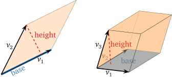
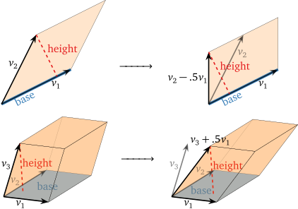
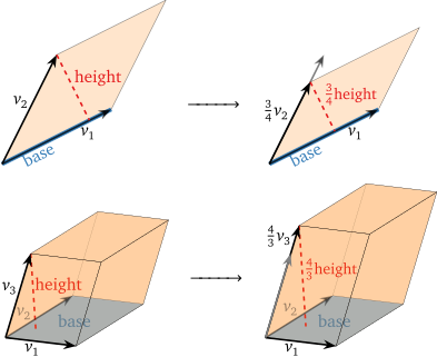
간단히 하기 위해 $R_n = R_n + cR_i$ 꼴의 행 대체를 생각합니다. 평행육면체의 부피는 밑면의 부피에 높이를 곱한 것입니다: 여기서 “밑면”은 $v_1,v_2,\ldots,v_{n-1}$ 로 결정되는 평행육면체이고, “높이”는 밑면으로부터 $v_n$ 까지의 수직 거리입니다.
$\begin{tikzpicture}[thin border nodes, scale=1.3] \filldraw[fill=seq-orange, fill opacity=.2, very thin] (0,0) -- (1,2) -- (3,3) -- (2,1) -- cycle; \draw[line width=1mm, seq-blue] (0,0) to["base"' {pos=.3,sloped}] (2,1); \draw[vector] (0,0) -- node[auto]{$v_2$} (1,2); \draw[vector, opacity=.75] (0,0) -- node[auto,swap,opacity=1,pos=.7]{$v_1$} (2,1); \draw[dashed, very thick, seq-red] (1,2) to["height"] (8/5,4/5); \end{tikzpicture} \qquad \begin{tikzpicture}[thin border nodes, myxyz, scale=2] \filldraw[fill=seq-orange, opacity=.2, very thin] (0,0,0) -- (-1,0,0) -- (-1,.3,1) -- (0,.3,1) -- cycle; \filldraw[fill=seq-blue, opacity=.5, very thin] (0,0,0) -- (-1,0,0) -- (-.8,1,0) -- (.2,1,0) -- cycle; \node[seq-blue] at (-.4,.5,0) {base}; \filldraw[fill=seq-orange, opacity=.2, shift={(-1,0,0)}, very thin] (0,0,0) -- (.2,1,0) -- (.2,1.3,1) -- (0,.3,1) -- cycle; \draw[dashed, very thick, seq-red] (0,.3,1) to["height" pos=.55] (-.2,.2,0); \filldraw[fill=seq-orange, fill opacity=.2, very thin] (0,0,0) -- (.2,1,0) -- (.2,1.3,1) -- (0,.3,1) -- cycle; \filldraw[fill=seq-orange, fill opacity=.2, shift={(.2,1,0)}, very thin] (0,0,0) -- (-1,0,0) -- (-1,.3,1) -- (0,.3,1) -- cycle; \filldraw[fill=seq-orange, fill opacity=.2, shift={(0,.3,1)}, very thin] (0,0,0) -- (-1,0,0) -- (-.8,1,0) -- (.2,1,0) -- cycle; \draw[vector] (0,0,0) -- node[auto,swap] {$v_1$} (.2,1,0); \draw[vector, opacity=.4] (0,0,0) -- node[auto,pos=.4] {$v_2$} (-1,0,0); \draw[vector] (0,0,0) -- node[auto] {$v_3$} (0,.3,1); \end{tikzpicture}$
$v_n$ 을 $v_i$ 의 배수만큼 평행이동하면 $v_n$ 은 밑면과 평행한 방향으로 움직입니다. 이렇게 해도 밑면과 높이는 모두 변하지 않습니다! 따라서 $\vol(A)$ 는 행 대체에 의해 변하지 않습니다.
$\begin{tikzpicture}[thin border nodes, scale=1.3, baseline=1.3cm] \filldraw[fill=seq-orange, fill opacity=.2, very thin] (0,0) -- (1,2) -- (3,3) -- (2,1) -- cycle; \draw[line width=1mm, seq-blue] (0,0) to["base"' {pos=.3,sloped}] (2,1); \draw[vector] (0,0) -- node[auto]{$v_2$} (1,2); \draw[vector, opacity=.75] (0,0) -- node[auto,swap,opacity=1,pos=.7]{$v_1$} (2,1); \draw[dashed, very thick, seq-red] (1,2) to["height"] (8/5,4/5); \end{tikzpicture} $\quad\xrightarrow{\phantom{MMMM}}\quad$ \begin{tikzpicture}[thin border nodes, scale=1.3, baseline=1.3cm] \filldraw[fill=seq-orange, fill opacity=.2, very thin] (0,0) -- (0,3/2) -- (2,5/2) -- (2,1) -- cycle; \draw[line width=1mm, seq-blue] (0,0) to["base"' {pos=.3,sloped}] (2,1); \draw[vector, opacity=.5] (0,0) -- node[auto,swap,pos=.8]{$v_2$} (1,2); \draw[vector] (0,0) -- node[auto]{$v_2-.5v_1$} (0,3/2); \draw[vector, opacity=.75] (0,0) -- node[auto,swap,opacity=1,pos=.7]{$v_1$} (2,1); \draw[dashed, very thick, seq-red] (0,3/2) to["height"] (3/5,3/10); \end{tikzpicture}\\[3mm] \begin{tikzpicture}[thin border nodes, myxyz, scale=2, baseline=1.3cm] \filldraw[fill=seq-orange, opacity=.2, very thin] (0,0,0) -- (-1,0,0) -- (-1,.3,1) -- (0,.3,1) -- cycle; \filldraw[fill=seq-blue, opacity=.5, very thin] (0,0,0) -- (-1,0,0) -- (-.8,1,0) -- (.2,1,0) -- cycle; \node[seq-blue] at (-.4,.5,0) {base}; \filldraw[fill=seq-orange, opacity=.2, shift={(-1,0,0)}, very thin] (0,0,0) -- (.2,1,0) -- (.2,1.3,1) -- (0,.3,1) -- cycle; \draw[dashed, very thick, seq-red] (0,.3,1) to["height" pos=.55] (-.2,.2,0); \filldraw[fill=seq-orange, fill opacity=.2, very thin] (0,0,0) -- (.2,1,0) -- (.2,1.3,1) -- (0,.3,1) -- cycle; \filldraw[fill=seq-orange, fill opacity=.2, shift={(.2,1,0)}, very thin] (0,0,0) -- (-1,0,0) -- (-1,.3,1) -- (0,.3,1) -- cycle; \filldraw[fill=seq-orange, fill opacity=.2, shift={(0,.3,1)}, very thin] (0,0,0) -- (-1,0,0) -- (-.8,1,0) -- (.2,1,0) -- cycle; \draw[vector] (0,0,0) -- node[auto,swap] {$v_1$} (.2,1,0); \draw[vector, opacity=.4] (0,0,0) -- node[auto,pos=.4] {$v_2$} (-1,0,0); \draw[vector] (0,0,0) -- node[auto] {$v_3$} (0,.3,1); \end{tikzpicture} $\quad\xrightarrow{\phantom{MMMM}}\quad$ \begin{tikzpicture}[thin border nodes, myxyz, scale=2, baseline=1.3cm] \def\va{(.2,1,0)} \def\vb{(-1,0,0)} \def\vc{(.1,.8,1)} \tikzmath{ coordinate \vab; coordinate \vac; coordinate \vbc; \vab = \va + \vb; \vac = \va + \vc; \vbc = \vb + \vc; } \filldraw[fill=seq-orange, opacity=.2, very thin] (0,0,0) -- \vb -- (\vbc) -- \vc -- cycle; \filldraw[fill=seq-blue, opacity=.5, very thin] (0,0,0) -- \vb -- (\vab) -- \va -- cycle; \node[seq-blue] at (-.25,.35,0) {base}; \filldraw[fill=seq-orange, opacity=.2, shift={\vb}, very thin] (0,0,0) -- \va -- (\vac) -- \vc -- cycle; \draw[dashed, very thick, seq-red] \vc to["height" pos=.55] ($(-.2,.2,0)+.5*(.2,1,0)$); \filldraw[fill=seq-orange, fill opacity=.2, very thin] (0,0,0) -- \va -- (\vac) -- \vc -- cycle; \filldraw[fill=seq-orange, fill opacity=.2, shift={\va}, very thin] (0,0,0) -- \vb -- (\vbc) -- \vc -- cycle; \filldraw[fill=seq-orange, fill opacity=.2, shift={\vc}, very thin] (0,0,0) -- \vb -- (\vab) -- \va -- cycle; \draw[vector] (0,0,0) -- node[auto,swap] {$v_1$} \va; \draw[vector, opacity=.4] (0,0,0) -- node[auto,pos=.8] {$v_2$} \vb; \draw[vector] (0,0,0) -- \vc node[above] {$v_3+.5v_1$}; \draw[vector, opacity=.5] (0,0,0) -- node[auto,pos=.5] {$v_3$} (0,.3,1); \end{tikzpicture}$
간단히 하기 위해 $R_n = cR_n.$ 꼴의 행 스케일링을 생각합니다. 이는 $v_n$ 의 길이를 $|c|$ 배 하며, 따라서 밑면으로부터 $v_n$ 까지의 수직 거리도 $|c|$ 배 합니다. 따라서 $\vol(A)$ 는 $|c|$ 배가 됩니다.
$\begin{tikzpicture}[thin border nodes, scale=1.3, baseline=1.3cm] \filldraw[fill=seq-orange, fill opacity=.2, very thin] (0,0) -- (1,2) -- (3,3) -- (2,1) -- cycle; \draw[line width=1mm, seq-blue] (0,0) to["base"' {pos=.3, sloped}] (2,1); \draw[vector] (0,0) -- node[auto]{$v_2$} (1,2); \draw[vector, opacity=.75] (0,0) -- node[auto,swap,opacity=1,pos=.7]{$v_1$} (2,1); \draw[dashed, very thick, seq-red] (1,2) to["height"] (8/5,4/5); \end{tikzpicture} $\quad\xrightarrow{\phantom{MMMM}}\quad$ \begin{tikzpicture}[thin border nodes, scale=1.3, baseline=1.3cm] \filldraw[fill=seq-orange, fill opacity=.2, very thin] (0,0) -- (.75,1.5) -- (2.75,2.5) -- (2,1) -- cycle; \draw[line width=1mm, seq-blue] (0,0) to["base"' {pos=.3, sloped}] (2,1); \draw[vector, opacity=.5] (0,0) -- (1,2); \draw[vector] (0,0) -- node[auto]{$\frac34v_2$} (.75,1.5); \draw[vector, opacity=.75] (0,0) -- node[auto,swap,opacity=1,pos=.7]{$v_1$} (2,1); \draw[dashed, very thick, seq-red] (.75,1.5) to["$\frac34$\small height"] ($.75*(8/5,4/5)$); \end{tikzpicture}\\[3mm] \begin{tikzpicture}[thin border nodes, myxyz, scale=2, baseline=1.3cm] \filldraw[fill=seq-orange, opacity=.2, very thin] (0,0,0) -- (-1,0,0) -- (-1,.3,1) -- (0,.3,1) -- cycle; \filldraw[fill=seq-blue, opacity=.5, very thin] (0,0,0) -- (-1,0,0) -- (-.8,1,0) -- (.2,1,0) -- cycle; \node[seq-blue] at (-.4,.5,0) {base}; \filldraw[fill=seq-orange, opacity=.2, shift={(-1,0,0)}, very thin] (0,0,0) -- (.2,1,0) -- (.2,1.3,1) -- (0,.3,1) -- cycle; \draw[dashed, very thick, seq-red] (0,.3,1) to["height" pos=.55] (-.2,.2,0); \filldraw[fill=seq-orange, fill opacity=.2, very thin] (0,0,0) -- (.2,1,0) -- (.2,1.3,1) -- (0,.3,1) -- cycle; \filldraw[fill=seq-orange, fill opacity=.2, shift={(.2,1,0)}, very thin] (0,0,0) -- (-1,0,0) -- (-1,.3,1) -- (0,.3,1) -- cycle; \filldraw[fill=seq-orange, fill opacity=.2, shift={(0,.3,1)}, very thin] (0,0,0) -- (-1,0,0) -- (-.8,1,0) -- (.2,1,0) -- cycle; \draw[vector] (0,0,0) -- node[auto,swap] {$v_1$} (.2,1,0); \draw[vector, opacity=.4] (0,0,0) -- node[auto,pos=.4] {$v_2$} (-1,0,0); \draw[vector] (0,0,0) -- node[auto] {$v_3$} (0,.3,1); \end{tikzpicture} $\quad\xrightarrow{\phantom{MMMM}}\quad$ \begin{tikzpicture}[thin border nodes, myxyz, scale=2, baseline=1.3cm] \def\va{(.2,1,0)} \def\vb{(-1,0,0)} \def\vc{(0,.4,4/3)} \tikzmath{ coordinate \vab; coordinate \vac; coordinate \vbc; \vab = \va + \vb; \vac = \va + \vc; \vbc = \vb + \vc; } \filldraw[fill=seq-orange, opacity=.2, very thin] (0,0,0) -- \vb -- (\vbc) -- \vc -- cycle; \filldraw[fill=seq-blue, opacity=.5, very thin] (0,0,0) -- \vb -- (\vab) -- \va -- cycle; \node[seq-blue] at (-.4,.5,0) {base}; \filldraw[fill=seq-orange, opacity=.2, shift={\vb}, very thin] (0,0,0) -- \va -- (\vac) -- \vc -- cycle; \draw[dashed, very thick, seq-red] \vc to["$\frac43$\small height" pos=.55] ($4/3*(-.2,.2,0)$); \filldraw[fill=seq-orange, fill opacity=.2, very thin] (0,0,0) -- \va -- (\vac) -- \vc -- cycle; \filldraw[fill=seq-orange, fill opacity=.2, shift={\va}, very thin] (0,0,0) -- \vb -- (\vbc) -- \vc -- cycle; \filldraw[fill=seq-orange, fill opacity=.2, shift={\vc}, very thin] (0,0,0) -- \vb -- (\vab) -- \va -- cycle; \draw[vector] (0,0,0) -- node[auto,swap] {$v_1$} \va; \draw[vector, opacity=.4] (0,0,0) -- node[auto,pos=.5] {$v_2$} \vb; \draw[vector] (0,0,0) -- node[auto,pos=.8] {$\frac 43v_3$} \vc; \draw[vector, black!50!white] (0,0,0) -- (0,.3,1); \end{tikzpicture}$
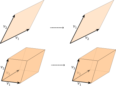
$A$ 의 두 행을 맞바꾸는 것은 벡터 $v_1,v_2,\ldots,v_n$ 의 순서를 바꿀 뿐이므로, 이 벡터들로 결정되는 평행육면체에는 아무런 영향을 주지 않습니다. 따라서 $\vol(A)$ 는 행 교환에 의해 변하지 않습니다.
$\begin{tikzpicture}[thin border nodes, scale=1.3, baseline=1.3cm] \filldraw[fill=seq-orange, fill opacity=.2, very thin] (0,0) -- (1,2) -- (3,3) -- (2,1) -- cycle; \draw[vector] (0,0) -- node[auto]{$v_2$} (1,2); \draw[vector] (0,0) -- node[auto,swap]{$v_1$} (2,1); \end{tikzpicture} $\quad\xrightarrow{\phantom{MMMM}}\quad$ \begin{tikzpicture}[thin border nodes, scale=1.3, baseline=1.3cm] \filldraw[fill=seq-orange, fill opacity=.2, very thin] (0,0) -- (1,2) -- (3,3) -- (2,1) -- cycle; \draw[vector] (0,0) -- node[auto]{$v_1$} (1,2); \draw[vector] (0,0) -- node[auto,swap]{$v_2$} (2,1); \end{tikzpicture}\\[3mm] \begin{tikzpicture}[thin border nodes, myxyz, scale=2, baseline=1.3cm] \filldraw[fill=seq-orange, opacity=.2, very thin] (0,0,0) -- (-1,0,0) -- (-1,.3,1) -- (0,.3,1) -- cycle; \filldraw[fill=seq-orange, opacity=.2, very thin] (0,0,0) -- (-1,0,0) -- (-.8,1,0) -- (.2,1,0) -- cycle; \filldraw[fill=seq-orange, opacity=.2, shift={(-1,0,0)}, very thin] (0,0,0) -- (.2,1,0) -- (.2,1.3,1) -- (0,.3,1) -- cycle; \filldraw[fill=seq-orange, fill opacity=.2, very thin] (0,0,0) -- (.2,1,0) -- (.2,1.3,1) -- (0,.3,1) -- cycle; \filldraw[fill=seq-orange, fill opacity=.2, shift={(.2,1,0)}, very thin] (0,0,0) -- (-1,0,0) -- (-1,.3,1) -- (0,.3,1) -- cycle; \filldraw[fill=seq-orange, fill opacity=.2, shift={(0,.3,1)}, very thin] (0,0,0) -- (-1,0,0) -- (-.8,1,0) -- (.2,1,0) -- cycle; \draw[vector] (0,0,0) -- node[auto,swap] {$v_1$} (.2,1,0); \draw[vector, opacity=.4] (0,0,0) -- node[auto] {$v_3$} (-1,0,0); \draw[vector] (0,0,0) -- node[auto] {$v_2$} (0,.3,1); \end{tikzpicture} $\quad\xrightarrow{\phantom{MMMM}}\quad$ \begin{tikzpicture}[thin border nodes, myxyz, scale=2, baseline=1.3cm] \filldraw[fill=seq-orange, opacity=.2, very thin] (0,0,0) -- (-1,0,0) -- (-1,.3,1) -- (0,.3,1) -- cycle; \filldraw[fill=seq-orange, opacity=.2, very thin] (0,0,0) -- (-1,0,0) -- (-.8,1,0) -- (.2,1,0) -- cycle; \filldraw[fill=seq-orange, opacity=.2, shift={(-1,0,0)}, very thin] (0,0,0) -- (.2,1,0) -- (.2,1.3,1) -- (0,.3,1) -- cycle; \filldraw[fill=seq-orange, fill opacity=.2, very thin] (0,0,0) -- (.2,1,0) -- (.2,1.3,1) -- (0,.3,1) -- cycle; \filldraw[fill=seq-orange, fill opacity=.2, shift={(.2,1,0)}, very thin] (0,0,0) -- (-1,0,0) -- (-1,.3,1) -- (0,.3,1) -- cycle; \filldraw[fill=seq-orange, fill opacity=.2, shift={(0,.3,1)}, very thin] (0,0,0) -- (-1,0,0) -- (-.8,1,0) -- (.2,1,0) -- cycle; \draw[vector] (0,0,0) -- node[auto,swap] {$v_1$} (.2,1,0); \draw[vector, opacity=.4] (0,0,0) -- node[auto] {$v_2$} (-1,0,0); \draw[vector] (0,0,0) -- node[auto] {$v_3$} (0,.3,1); \end{tikzpicture}$
단위행렬 $I_n$ 의 행들은 표준 좌표 벡터 $e_1,e_2,\ldots,e_n$ 입니다. 이에 대응하는 평행육면체는 단위 정육면체이며, 그 부피는 $1$ 입니다. 따라서 $\vol(I_n) = 1$ 입니다.

$|\det|$ 는 이러한 성질을 만족하는 유일한 함수이므로 다음이 성립합니다.

$\begin{equation*} \vol(P) = \vol(A) = |\det(A)|. \end{equation*}$

이로써 증명이 끝납니다.

전치 성질에 의해 $\det(A) = \det(A^T)$ 이므로, $\det(A)$ 의 절댓값은 $A$ 의 열들로 결정되는 평행육면체의 부피와도 같습니다.

예제(길이)

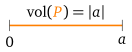
$1\times 1$ 행렬 $A$ 는 단지 하나의 수 $\mat a$ 입니다. 이 경우 하나뿐인 행이 결정하는 평행육면체 $P$ 는 단지 구간 $[0,a]$ ( $a\lt0$ 이면 $[a,0]$ )입니다. $\R^1 = \R$ 에서 영역의 “부피”는 단지 그 길이이므로, 이 경우 $\vol(P) = |a|$ 임은 분명합니다.

$\begin{tikzpicture} \draw[very thick, draw=seq-orange] (0,0) -- node[above] {$\vol(\textcolor{seq-orange}{P}) = |a|$} (3,0); \draw (0,.15) -- (0,-.15) node[below] {$0$} (3,.15) -- (3,-.15) node[below] {$a$}; \end{tikzpicture}$

예제(넓이)

$A$ 가 $2\times 2$ 행렬이면, 그 행들은 $\R^2$ 에서 평행사변형을 결정합니다. $\R^2$ 에서 영역의 “부피”는 그 넓이이므로, 평행사변형의 넓이에 대한 공식을 얻습니다. 즉, 평행사변형의 넓이는 평행사변형의 이웃한 두 변을 이루는 벡터들을 행으로 갖는 행렬의 행렬식입니다.

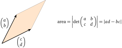
$\begin{tikzpicture}[thin border nodes, scale=1.3] \filldraw[fill=seq-orange, fill opacity=.2, very thin] (0,0) -- (1,2) -- (3,3) -- (2,1) -- cycle; \draw[vector] (0,0) -- node[auto]{$\vec{a b}$} (1,2); \draw[vector] (0,0) -- node[auto,swap,opacity=1]{$\vec{c d}$} (2,1); \node at (6, 1.5) {area${}=\left|\det\mat{a b; c d}\right| = |ad-bc|$}; \end{tikzpicture}$

삼각법 없이 평행사변형의 넓이를 계산할 수 있다는 것은 어쩌면 놀라운 일입니다. 이 공식을 직접 증명해 보는 것은 재미있는 기하 문제입니다. [힌트: 먼저 $A$ 의 첫 번째 행이 $x$ -축 위에 놓이는 경우를 생각해 보십시오.]

예제

예제(삼각형의 넓이)

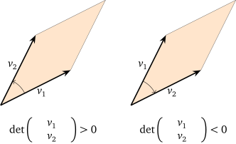
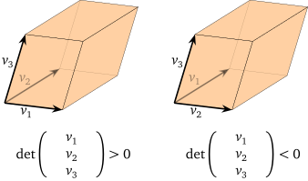
행렬식의 절댓값이 부피라면, 절댓값을 취하지 않은 행렬식의 기하학적 의미는 무엇인지 궁금할 수도 있습니다. 다음 참고에서는 행렬식을 부호가 있는 부피로 생각할 수 있음을 설명합니다. 적분학 강의를 들었다면 곡선 아래의 음의 넓이를 계산해 보았을 것입니다. 여기서의 생각도 그와 비슷합니다.

참고(부호가 있는 부피)

소절4.3.3영역의 부피

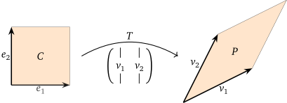
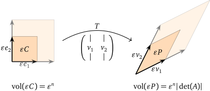
$A$ 를 열이 $v_1,v_2,\ldots,v_n$ 인 $n\times n$ 행렬이라 하고, $T\colon\R^n\to\R^n$ 를 이에 대응하는 행렬 변환 $T(x)=Ax$ 라 합시다. 그러면 $T(e_1)=v_1$ 이고 $T(e_2)=v_2$ 이므로, $T$ 는 단위 정육면체 $C$ 를 $v_1,v_2,\ldots,v_n$ 가 결정하는 평행육면체 $P$ 로 보냅니다:

$\begin{tikzpicture}[thin border nodes, scale=1.3] \begin{scope}[scale=1.7, yshift=.3cm] \filldraw[fill=seq-orange, fill opacity=.2, very thin] (0,0) -- (1,0) -- (1,1) -- (0,1) -- cycle; \node at (.5, .5) {$C$}; \draw[vector] (0,0) -- node[auto]{$e_2$} (0,1); \draw[vector, opacity=.75] (0,0) -- node[auto,swap]{$e_1$} (1,0); \coordinate (a) at (1.2, .5); \end{scope} \draw[->, thick] (a) to[bend left] node[above=2pt] {$T$} node[below=4pt] {$\mat{| |; v_1 v_2; | |}$} ($(a) + (2.8cm,0)$); \begin{scope}[xshift=5cm] \filldraw[fill=seq-orange, fill opacity=.2, very thin] (0,0) -- (1,2) -- (3,3) -- (2,1) -- cycle; \draw[vector] (0,0) -- node[auto]{$v_2$} (1,2); \draw[vector] (0,0) -- node[auto,swap]{$v_1$} (2,1); \node at (1.5, 1.5) {$P$}; \end{scope} \end{tikzpicture}$

단위 정육면체의 부피는 $1$ 이고 그 상의 부피는 $|\det(A)|$ 이므로, 변환 $T$ 는 정육면체의 부피를 $|\det(A)|$ 배로 바꾼 것입니다. 다시 말하면 다음과 같습니다.

$A$ 가 $n\times n$ 행렬이고 이에 대응하는 행렬 변환이 $T\colon\R^n\to\R^n$ 이며 $C$ 가 $\R^n$ 의 단위 정육면체이면, $T(C)$ 의 부피는 다음과 같습니다: $|\det(A)|.$

$T(S)$ 라는 표기는 변환 $T$ 에 의한 영역 $S$ 의 상을 뜻합니다. 조건제시법으로 나타내면 이는 다음 부분집합입니다.

$\begin{equation*} T(S) = \bigl\{T(x)\mid x \text{ in } S\bigr\}. \end{equation*}$

사실 $T$ 는 $\R^n$ 의 임의의 영역의 부피를 같은 배율로 바꾸며, 이는 곡선으로 둘러싸인 영역에서도 마찬가지입니다.

정리

$A$ 를 $n\times n$ 행렬이라 하고, $T\colon\R^n\to\R^n$ 를 이에 대응하는 행렬 변환 $T(x)=Ax$ 라 합시다. $S$ 가 $\R^n$ 의 임의의 영역이면 다음이 성립합니다.

$\begin{equation*} \vol(T(S))=|\det(A)|\cdot\vol(S). \end{equation*}$

증명

$C$ 를 단위 정육면체라 하고, $v_1,v_2,\ldots,v_n$ 를 $A$ 의 열이라 하며, $P$ 를 이 벡터들이 결정하는 평행육면체라 하면 $T(C) = P$ 이고 $\vol(P) = |\det(A)|$ 입니다. $\epsilon > 0$ 에 대해 $\epsilon C$ 를 변의 길이가 $\epsilon$ 인 정육면체, 즉 벡터 $\epsilon e_1,\epsilon e_2,\ldots,\epsilon e_n$ 가 결정하는 평행육면체라 하고, $\epsilon P$ 도 같은 방식으로 정의합니다. 두 번째 정의 성질에 의해 $T$ 는 $\epsilon C$ 를 $\epsilon P$ 로 보냅니다. $\epsilon C$ 의 부피는 $\epsilon^n$ 이고( $n$ 개의 표준 벡터 각각을 $\epsilon$ 배 했기 때문입니다) $\epsilon P$ 의 부피는 $\epsilon^n|\det(A)|$ 이므로(같은 이유입니다), $T$ 가 $\epsilon C$ 의 부피를 $|\det(A)|$ 배로 바꾼다는 것을 보였습니다.

$\begin{tikzpicture}[thin border nodes, scale=1.3] \begin{scope}[scale=1.7, yshift=.3cm] \filldraw[very thin, black!50!white, fill=seq-orange!10!white] (0,0) -- (1,0) -- (1,1) -- (0,1) -- cycle; \filldraw[fill=seq-orange, fill opacity=.2, very thin] (0,0) -- (.6,0) -- (.6,.6) -- (0,.6) -- cycle; \draw[vector, black!50!white] (0, 0) -- (1, 0); \draw[vector, black!50!white] (0, 0) -- (0, 1); \draw[vector] (0,0) -- node[auto]{$\epsilon e_2$} (0,.6); \draw[vector, opacity=.75] (0,0) -- node[auto,swap]{$\epsilon e_1$} (.6,0); \node at (.3, .3) {$\epsilon C$}; \coordinate (a) at (1.2, .5); \end{scope} \node at (1.7/2, -.5) {$\vol(\epsilon C) = \epsilon^n$}; \draw[->, thick] (a) to[bend left] node[above=2pt] {$T$} node[below=4pt] {$\mat{| |; v_1 v_2; | |}$} ($(a) + (2.8cm,0)$); \begin{scope}[xshift=5cm] \filldraw[black!50!white, fill=seq-orange!10!white, very thin] (0,0) -- (1,2) -- (3,3) -- (2,1) -- cycle; \filldraw[fill=seq-orange, fill opacity=.2, very thin] (0,0) -- (.6,1.2) -- (1.8,1.8) -- (1.2,.6) -- cycle; \draw[vector, black!50!white] (0, 0) -- (1,2); \draw[vector, black!50!white] (0, 0) -- (2,1); \draw[vector] (0,0) -- node[auto]{$\epsilon v_2$} (.6,1.2); \draw[vector] (0,0) -- node[auto,swap]{$\epsilon v_1$} (1.2,.6); \node at (.9,.9) {$\epsilon P$}; \end{scope} \node at (6.3, -.5) {$\vol(\epsilon P) = \epsilon^n|\det(A)|$}; \end{tikzpicture}$

첫 번째 정의 성질에 의해 $\epsilon C$ 를 평행이동한 것의 상은 $\epsilon P$ 를 평행이동한 것입니다:

$\begin{equation*} T(x + \epsilon C) = T(x) + \epsilon T(C) = T(x) + \epsilon P. \end{equation*}$

평행이동은 부피를 바꾸지 않으므로, 이로써 $T$ 가 $\epsilon C$ 를 평행이동한 것의 부피를 $|\det(A)|$ 배로 바꾼다는 것이 증명됩니다.

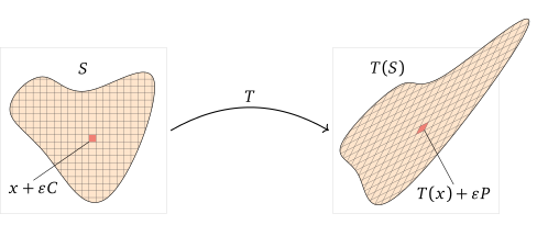
여기서부터는 다변수 미적분학의 기법을 사용해야 하므로, 나머지 증명은 아이디어만 제시합니다. 임의의 영역 $S$ 는 $x + \epsilon C$ 꼴의 매우 작은 정육면체들의 모임으로 근사할 수 있습니다. 그러면 상 $T(S)$ 는 이 정육면체 모임의 상으로 근사되며, 이는 $T(x) + \epsilon P$ 꼴의 매우 작은 평행육면체들의 모임입니다.

$\def\curvy{(-37.3333, 2.6667) .. controls (-37.3333, -5.3333) and (-26.6667, -10.6667) .. (-16, -24) .. controls (-5.3333, -37.3333) and (5.3333, -58.6667) .. (18.6667, -48) .. controls (32, -37.3333) and (48, 5.3333) .. (45.3333, 18.6667) .. controls (42.6667, 32) and (21.3333, 16) .. (8, 13.3333) .. controls (-5.3333, 10.6667) and (-10.6667, 21.3333) .. (-18.6667, 21.3333) .. controls (-26.6667, 21.3333) and (-37.3333, 10.6667) .. cycle} \begin{tikzpicture}[scale=1, thin border nodes] \draw[help lines, black!25] (-2,-2) rectangle (2,2); \begin{scope}[fill=seq-orange, fill opacity=.2, thin, x=1.7*.7bp, y=1.7*.7bp, yshift=.4cm, xshift=-.2cm] \expandafter\filldraw\curvy; \expandafter\clip\curvy; \fill[seq-red, opacity=.5, shift={(2*4,-4*4)}] (0,0) rectangle (4,4); \coordinate (a) at (2*4,-4*4); \draw[very thin, black!70!white, step=4] (-60,-60) grid (60,60); \end{scope} \draw[thin] (-1.2, -1.2) node[below] {$x + \epsilon C$} -- (a); \node at (0,1.5) {$S$}; %\point at (0,0); \draw[->, thick] (2.1,0) to[bend left, "$T$" above=1mm] (8-2.1,0); \begin{scope}[xshift=8cm] \draw[help lines, black!25] (-2,-2) rectangle (2,2); \begin{scope}[cm={2,1,1,2,(0,.5)}, x=.7bp, y=.7bp, fill=seq-orange, fill opacity=.2, thin] \expandafter\filldraw\curvy; \expandafter\clip\curvy; \fill[seq-red, opacity=.5, shift={(2*4,-4*4)}] (0,0) rectangle (4,4); \draw[very thin, black!70!white, step=4] (-60,-60) grid (60,60); \coordinate (b) at (3*4,-4*4); \end{scope} \draw[thin] (.9,-1.3) node[below] {$T(x) + \epsilon P$} -- (b); \node at (-.7,1.5) {$T(S)$}; % \point at (0,0); \end{scope} \end{tikzpicture}$

$S$ 의 부피는 정육면체들의 부피의 합으로 가깝게 근사되며, 실제로 $\epsilon$ 이 0으로 갈 때 이 합의 극한은 정확히 $\vol(S)$ 입니다. 마찬가지로 $T(S)$ 의 부피는 $\epsilon\to 0$ 일 때의 극한을 취한 평행육면체들의 부피의 합과 같습니다. 핵심은 다음과 같습니다. 각 정육면체의 부피는 $|\det(A)|$ 배가 됩니다. 따라서 평행육면체들의 부피의 합은 정육면체들의 부피의 합의 $|\det(A)|$ 배입니다. 이로써 다음이 증명됩니다: $\vol(T(S)) = |\det(A)|\vol(S).$