절2.9랭크 정리¶ 고유 링크

목표

랭크 정리를 이해하고 활용하는 법을 익힙니다.
그림: 랭크 정리.
정리: 랭크 정리.
용어: 랭크, 퇴화차수.

이 절에서는 지금까지 해 온 모든 작업의 정점인 랭크 정리를 소개합니다.

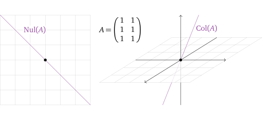
독자는 행렬의 열공간과 영공간 사이에 어떤 관계가 있음을 눈치챘을 수도 있습니다. 이 예제 in 절 2.6에서 $3\times 2$ 행렬의 열공간과 영공간은 둘 다 직선이며, 각각 $\R^2$ 와 $\R^3$ 에 놓여 있습니다:

$\begin{tikzpicture}[myxyz, scale=.8] \begin{scope}[resetxy] \draw[grid lines] (-3,-3) grid (3,3); \draw[seq4] (-3,3) -- (3,-3); \point at (0,0); \node[seq4,fill=white, inner sep=1pt] at (-.7,2) {$\Nul(A)$}; \end{scope} \begin{scope}[xshift=9cm] \path[clip, resetxy] (-6,-4) rectangle (6,4); \def\v{(1, 1, 1)} \node[coordinate] (X) at \v {}; \draw[seq4] (0,0,0) -- ($-6*(X)$); \draw (0,0,-3) -- (0,0,0); \begin{scope}[transformxy] \fill[white, nearly opaque] (-3, -3) rectangle (3, 3); \draw[grid lines] (-3, -3) grid (3, 3); \draw[->] (-3,0) -- (3,0); \draw[->] (0,-3) -- (0,3); \end{scope} \draw[seq4] (0,0,0) -- node[right, pos=.7] {$\Col(A)$} ($6*(X)$); \draw[->] (0,0,0) -- (0,0,3); \point at (0,0,0); \end{scope} \node[fill=white, resetxy] at (5, 2) {$A = \mat{1 1; 1 1; 1 1}$}; \end{tikzpicture}$

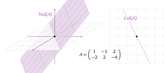
이 예제 in 절 2.4에서 $2\times 3$ 행렬 $\bigl(\begin{smallmatrix}1&-1&2\\-2&2&-4\end{smallmatrix}\bigr)$ 의 영공간은 $\R^3$ 의 평면이고, 열공간은 ${1\choose-2}$ 가 생성하는 $\R^2$ 의 직선입니다:

$\begin{tikzpicture}[myxyz, scale=.8] \begin{scope}[xshift=9cm, resetxy] \draw[grid lines] (-3,-3) grid (3,3); \draw[seq4] (-1.5,3) -- (1.5,-3); \point at (0,0); \node[seq4,fill=white, inner sep=1pt] at (-.7,2) {$\Col(A)$}; \end{scope} \begin{scope} \path[clip, resetxy] (-6,-4) rectangle (6,4); \def\v{(1, 1, 0)} \def\w{(-2, 0, 1)} \node[coordinate] (X) at \v {}; \node[coordinate] (Y) at \w {}; \draw (0,0,-3) -- (0,0,0); \begin{scope}[x=(X), y=(Y), transformxy] \path[clip] (-5, 0) -- (-5, -5) -- (5, -5) -- (5, 0) -- cycle; \fill[seq4!30, nearly opaque] (-3,-2) rectangle (3,2); \draw[step=1cm, seq4, very thin] (-3,-2) grid (3,2); \end{scope} \begin{scope}[transformxy] \fill[white, nearly opaque] (-3, -3) rectangle (3, 3); \draw[grid lines] (-3, -3) grid (3, 3); \draw[->] (-3,0) -- (3,0); \draw[->] (0,-3) -- (0,3); \end{scope} \begin{scope}[x=(X), y=(Y), transformxy] \path[clip] (-5, 0) -- (-5, 5) -- (5, 5) -- (5, 0) -- cycle; \fill[seq4!30, nearly opaque] (-3,-2) rectangle (3,2); \draw[step=1cm, seq4, very thin] (-3,-2) grid (3,2); \end{scope} \draw[->] (0,0,0) -- (0,0,3); \node[seq4, anchor=south east] at (-3,-2.5,.5) {$\Nul(A)$}; \point at (0,0,0); \end{scope} \node[fill=white, resetxy] at (5, -2) {$A = \mat{1 -1 2; -2 2 -4}$}; \end{tikzpicture}$

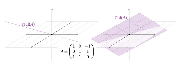
이 예제 in 절 2.4에서 $3\times 3$ 행렬의 영공간은 $\R^3$ 의 직선이고, 열공간은 $\R^3$ 의 평면입니다:

$\begin{tikzpicture}[myxyz, scale=.8] \begin{scope}[xshift=9cm] \path[clip, resetxy] (-6,-4) rectangle (6,4); \draw (0,0,-3) -- (0,0,0); \def\v{(1, 0, 1)} \def\w{(-1/2, 1, 1/2)} \node[coordinate] (X) at \v {}; \node[coordinate] (Y) at \w {}; \begin{scope}[x=(X), y=(Y), transformxy] \path[clip] (-5/2, 5) -- (-5, 5) -- (-5, -5) -- (5/2, -5) -- cycle; \fill[seq4!30, nearly opaque] (-2,-2) rectangle (2,2); \draw[step=1cm, seq4, very thin] (-2,-2) grid (2,2); \end{scope} \begin{scope}[transformxy] \fill[white, nearly opaque] (-3, -3) rectangle (3, 3); \draw[grid lines] (-3, -3) grid (3, 3); \draw[->] (-3,0) -- (3,0); \draw[->] (0,-3) -- (0,3); \end{scope} \begin{scope}[x=(X), y=(Y), transformxy] \path[clip] (-5/2, 5) -- (5, 5) -- (5, -5) -- (5/2, -5) -- cycle; \fill[seq4!30, nearly opaque] (-2,-2) rectangle (2,2); \draw[step=1cm, seq4, very thin] (-2,-2) grid (2,2); \end{scope} \draw[->] (0,0,0) -- (0,0,3); \node[seq4, anchor=south east] at (-3,-2.5,0) {$\Col(A)$}; \point at (0,0,0); \end{scope} \begin{scope} \path[clip, resetxy] (-6,-4) rectangle (6,4); \def\v{(1, -1, 1)} \node[coordinate] (X) at \v {}; \draw[seq4] (0,0,0) -- ($-3*(X)$); \draw (0,0,-3) -- (0,0,0); \begin{scope}[transformxy] \fill[white, nearly opaque] (-3, -3) rectangle (3, 3); \draw[grid lines] (-3, -3) grid (3, 3); \draw[->] (-3,0) -- (3,0); \draw[->] (0,-3) -- (0,3); \end{scope} \draw[seq4] (0,0,0) -- node[above] {$\Nul(A)$} ($3*(X)$); \draw[->] (0,0,0) -- (0,0,3); \point at (0,0,0); \end{scope} \node[fill=white, resetxy] at (3, -2) {$A = \mat{1 0 -1; 0 1 1; 1 1 0}$}; \end{tikzpicture}$

모든 예에서 열공간의 차원과 영공간의 차원을 더하면 행렬의 열의 개수와 같습니다. 이것이 바로 랭크 정리의 내용입니다.

정의

행렬 $A$ 의 랭크는 $\rank(A)$ 로 쓰며, 열공간 $\Col(A)$ 의 차원입니다.

행렬 $A$ 의 퇴화차수는 $\nullity(A)$ 로 쓰며, 영공간 $\Nul(A)$ 의 차원입니다.

행렬 $A$ 의 랭크는 $Ax=b$ 의 해에 관한 중요한 정보를 알려 줍니다. 이 참고 in 절 2.3에서 $Ax=b$ 는 $b$ 가 $A$ 의 열들의 생성 안에 있을 때, 다시 말해 $b$ 가 $A$ 의 열공간 안에 있을 때 정확히 일관적이라는 것을 떠올려 보십시오. 따라서 $\rank(A)$ 는 $Ax=b$ 가 일관적이 되게 하는 $b$ 들의 집합의 차원입니다.

$A$ 의 랭크는 피벗 열의 개수와 같고(이 정리 in 절 2.7 참조), $A$ 의 퇴화차수는 자유변수의 개수, 즉 피벗이 없는 열의 개수와 같다는 것을 우리는 알고 있습니다(이 정리 in 절 2.7 참조). 피벗 열과 자유변수에 관한 내용을 요약하면 다음과 같습니다:

$\begin{align*} \rank(A) = \dim\Col(A) &= \text{the number of columns with pivots}\\ \nullity(A) = \dim\Nul(A) &= \text{the number of free variables}\\ &= \text{the number of columns without pivots} \end{align*}$

분명히

$\begin{equation*} \text{\#(columns with pivots)} + \text{\#(columns without pivots)} = \text{\#(columns)}, \end{equation*}$

이므로 다음 정리를 증명하였습니다.

랭크 정리

$A$ 가 $n$ 개의 열을 가진 행렬이면 다음이 성립합니다.

$\begin{equation*} \rank(A) + \nullity(A) = n. \end{equation*}$

다시 말해, 해가 있는 임의의 연립일차방정식에 대하여 다음이 성립합니다.

$\begin{equation*} \text{(dim of column span)} + \text{(dim of solution set)} = \text{(number of variables)}. \end{equation*}$

랭크 정리는 우리의 주된 관심 대상인 두 가지, 즉 행렬의 영공간( $Ax=0$ 의 해집합)과 열공간( $Ax=b$ 를 일관적으로 만드는 벡터 $b$ 의 집합) 사이의 강한 관계를 보여 주므로, 실로 이 장의 정점이라 할 수 있습니다. $x$ 를 선택하는 자유도가 클수록 $b$ 를 선택하는 자유도는 작아지며, 그 반대도 마찬가지입니다.

예제(랭크와 퇴화차수)

랭크 정리는 선형대수학의 이론을 이용하여 연립방정식을 직접 풀지 않고도 그에 관해 정성적인 사실을 말할 수 있음을 보여 주는 대표적인 예입니다. 본질적으로 이것이 바로 이 학문의 힘입니다.

예제(랭크가 2이고 퇴화차수가 2인 경우)

인터랙티브: 랭크가 1이고 퇴화차수가 2인 경우

인터랙티브: 랭크가 2이고 퇴화차수가 1인 경우

번역에 대한 의견이나 오류 제보(GitHub 계정 필요)