Original

기초 기하학

이 글에서는 해석 기하학 전체의 기초를 이루는 유클리드 공간의 점에 대한 기본 연산을 살펴보겠습니다. 각 점 $\mathbf r$에 대해 $\mathbf 0$에서 $\mathbf r$로 향하는 벡터 $\vec{\mathbf r}$을 생각하겠습니다. 이후로는 $\mathbf r$과 $\vec{\mathbf r}$을 구분하지 않고, 점이라는 용어를 벡터의 동의어로 사용하겠습니다.

선형 연산

2D 점과 3D 점은 모두 선형 공간을 이룹니다. 즉, 점끼리의 합과 점에 어떤 수를 곱하는 곱셈이 정의되어 있습니다. 다음은 2차원에 대한 기본 구현입니다:

struct point2d {
    ftype x, y;
    point2d() {}
    point2d(ftype x, ftype y): x(x), y(y) {}
    point2d& operator+=(const point2d &t) {
        x += t.x;
        y += t.y;
        return *this;
    }
    point2d& operator-=(const point2d &t) {
        x -= t.x;
        y -= t.y;
        return *this;
    }
    point2d& operator*=(ftype t) {
        x *= t;
        y *= t;
        return *this;
    }
    point2d& operator/=(ftype t) {
        x /= t;
        y /= t;
        return *this;
    }
    point2d operator+(const point2d &t) const {
        return point2d(*this) += t;
    }
    point2d operator-(const point2d &t) const {
        return point2d(*this) -= t;
    }
    point2d operator*(ftype t) const {
        return point2d(*this) *= t;
    }
    point2d operator/(ftype t) const {
        return point2d(*this) /= t;
    }
};
point2d operator*(ftype a, point2d b) {
    return b * a;
}

그리고 3차원 점에 대한 구현입니다:

struct point3d {
    ftype x, y, z;
    point3d() {}
    point3d(ftype x, ftype y, ftype z): x(x), y(y), z(z) {}
    point3d& operator+=(const point3d &t) {
        x += t.x;
        y += t.y;
        z += t.z;
        return *this;
    }
    point3d& operator-=(const point3d &t) {
        x -= t.x;
        y -= t.y;
        z -= t.z;
        return *this;
    }
    point3d& operator*=(ftype t) {
        x *= t;
        y *= t;
        z *= t;
        return *this;
    }
    point3d& operator/=(ftype t) {
        x /= t;
        y /= t;
        z /= t;
        return *this;
    }
    point3d operator+(const point3d &t) const {
        return point3d(*this) += t;
    }
    point3d operator-(const point3d &t) const {
        return point3d(*this) -= t;
    }
    point3d operator*(ftype t) const {
        return point3d(*this) *= t;
    }
    point3d operator/(ftype t) const {
        return point3d(*this) /= t;
    }
};
point3d operator*(ftype a, point3d b) {
    return b * a;
}

여기서 ftype은 좌표에 사용하는 타입으로, 보통 int, double 또는 long long입니다.

내적

정의

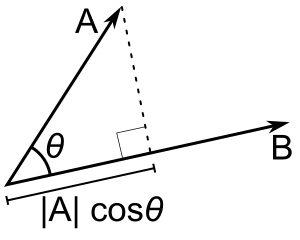
벡터 $\mathbf a$와 $\mathbf b$의 내적(또는 스칼라곱) $\mathbf a \cdot \mathbf b$는 동등한 두 가지 방식으로 정의할 수 있습니다. 기하학적으로는 첫 번째 벡터의 길이와 두 번째 벡터를 첫 번째 벡터에 사영한 길이의 곱입니다. 아래 그림에서 볼 수 있듯이 이 사영은 바로 $|\mathbf a| \cos \theta$이며, 여기서 $\theta$는 $\mathbf a$와 $\mathbf b$ 사이의 각입니다. 따라서 $\mathbf a\cdot \mathbf b = |\mathbf a| \cos \theta \cdot |\mathbf b|$입니다.

내적은 몇 가지 주목할 만한 성질을 가집니다:

1. $\mathbf a \cdot \mathbf b = \mathbf b \cdot \mathbf a$
2. $(\alpha \cdot \mathbf a)\cdot \mathbf b = \alpha \cdot (\mathbf a \cdot \mathbf b)$
3. $(\mathbf a + \mathbf b)\cdot \mathbf c = \mathbf a \cdot \mathbf c + \mathbf b \cdot \mathbf c$

즉, 내적은 교환 법칙이 성립하며 두 인자 각각에 대해 선형인 함수입니다. 단위 벡터를 다음과 같이 표기합시다

$$\mathbf e_x = \begin{pmatrix} 1 \\ 0 \\ 0 \end{pmatrix}, \mathbf e_y = \begin{pmatrix} 0 \\ 1 \\ 0 \end{pmatrix}, \mathbf e_z = \begin{pmatrix} 0 \\ 0 \\ 1 \end{pmatrix}.$$

이 표기법을 사용하면 벡터 $\mathbf r = (x;y;z)$를 $r = x \cdot \mathbf e_x + y \cdot \mathbf e_y + z \cdot \mathbf e_z$로 쓸 수 있습니다. 그리고 단위 벡터에 대해 다음이 성립하므로

$$\mathbf e_x\cdot \mathbf e_x = \mathbf e_y\cdot \mathbf e_y = \mathbf e_z\cdot \mathbf e_z = 1,\\ \mathbf e_x\cdot \mathbf e_y = \mathbf e_y\cdot \mathbf e_z = \mathbf e_z\cdot \mathbf e_x = 0$$

좌표로 나타내면 $\mathbf a = (x_1;y_1;z_1)$과 $\mathbf b = (x_2;y_2;z_2)$에 대해 다음이 성립함을 알 수 있습니다

$$\mathbf a\cdot \mathbf b = (x_1 \cdot \mathbf e_x + y_1 \cdot\mathbf e_y + z_1 \cdot\mathbf e_z)\cdot( x_2 \cdot\mathbf e_x + y_2 \cdot\mathbf e_y + z_2 \cdot\mathbf e_z) = x_1 x_2 + y_1 y_2 + z_1 z_2$$

이것은 내적의 대수적 정의이기도 합니다. 이로부터 내적을 계산하는 함수를 작성할 수 있습니다.

ftype dot(point2d a, point2d b) {
    return a.x * b.x + a.y * b.y;
}
ftype dot(point3d a, point3d b) {
    return a.x * b.x + a.y * b.y + a.z * b.z;
}

문제를 풀 때는 내적을 계산하는 데 대수적 정의를 사용해야 하지만, 이를 활용하려면 기하학적 정의와 성질을 염두에 두어야 합니다.

성질

내적을 통해 여러 기하학적 성질을 정의할 수 있습니다. 예를 들면 다음과 같습니다

1. $\mathbf a$의 노름(길이의 제곱): $|\mathbf a|^2 = \mathbf a\cdot \mathbf a$
2. $\mathbf a$의 길이: $|\mathbf a| = \sqrt{\mathbf a\cdot \mathbf a}$
3. $\mathbf a$를 $\mathbf b$에 사영한 길이: $\dfrac{\mathbf a\cdot\mathbf b}{|\mathbf b|}$
4. 벡터 사이의 각: $\arccos \left(\dfrac{\mathbf a\cdot \mathbf b}{|\mathbf a| \cdot |\mathbf b|}\right)$
5. 앞의 항목에서 두 벡터 사이의 각이 예각이면 내적은 양수이고, 둔각이면 음수이며, 두 벡터가 직교하면, 즉 직각을 이루면 0임을 알 수 있습니다.

이 함수들은 모두 차원의 수와 무관하므로 2D와 3D의 경우에 동일하다는 점에 유의하십시오:

ftype norm(point2d a) {
    return dot(a, a);
}
double abs(point2d a) {
    return sqrt(norm(a));
}
double proj(point2d a, point2d b) {
    return dot(a, b) / abs(b);
}
double angle(point2d a, point2d b) {
    return acos(dot(a, b) / abs(a) / abs(b));
}

다음 중요한 성질을 알아보기 위해 어떤 고정된 상수 $C$에 대해 $\mathbf r\cdot \mathbf a = C$를 만족하는 점 $\mathbf r$의 집합을 살펴봅시다. 이 점들의 집합은 $\mathbf a$ 위로의 사영이 점 $C \cdot \dfrac{\mathbf a}{|\mathbf a| ^ 2}$인 점들의 집합과 정확히 일치하며, 이 점들은 $\mathbf a$에 직교하는 초평면을 이룬다는 것을 알 수 있습니다. 아래 그림에서 2D에서의 벡터 $\mathbf a$와 함께, 그것과 같은 내적 값을 갖는 여러 벡터를 볼 수 있습니다:

2D에서 이 벡터들은 직선을 이루고, 3D에서는 평면을 이룹니다. 이 결과를 이용하면 2D에서 직선을 $\mathbf r\cdot \mathbf n=C$ 또는 $(\mathbf r - \mathbf r_0)\cdot \mathbf n=0$으로 정의할 수 있다는 점에 유의하십시오. 여기서 $\mathbf n$은 직선에 직교하는 벡터이고, $\mathbf r_0$는 직선 위에 이미 있는 임의의 벡터이며, $C = \mathbf r_0\cdot \mathbf n$입니다. 같은 방식으로 3D에서 평면을 정의할 수 있습니다.

외적

정의

아래 그림과 같이 3D 공간에서 세 벡터 $\mathbf a$, $\mathbf b$, $\mathbf c$가 평행육면체를 이루고 있다고 가정합시다:

이 평행육면체의 부피는 어떻게 계산하겠습니까? 학교에서 배운 대로 밑면의 넓이에 높이를 곱해야 하며, 높이는 $\mathbf a$를 밑면에 직교하는 방향으로 사영한 것입니다. 즉, $\mathbf b \times \mathbf c$를 $\mathbf b$와 $\mathbf c$ 모두에 직교하고 그 길이가 $\mathbf b$와 $\mathbf c$가 이루는 평행사변형의 넓이와 같은 벡터로 정의하면, $|\mathbf a\cdot (\mathbf b\times\mathbf c)|$는 평행육면체의 부피와 같아집니다. 일관성을 위해 $\mathbf b\times \mathbf c$는 항상 $\mathbf b\times \mathbf c$의 끝점에서 보았을 때 벡터 $\mathbf b$에서 벡터 $\mathbf c$로의 회전이 반시계 방향이 되도록 향한다고 하겠습니다(아래 그림 참고).

이것으로 벡터 $\mathbf b$와 $\mathbf c$의 외적(또는 벡터곱) $\mathbf b\times \mathbf c$와 벡터 $\mathbf a$, $\mathbf b$, $\mathbf c$의 삼중곱 $\mathbf a\cdot(\mathbf b\times \mathbf c)$가 정의됩니다.

외적과 삼중곱의 몇 가지 주목할 만한 성질은 다음과 같습니다:

1. $\mathbf a\times \mathbf b = -\mathbf b\times \mathbf a$
2. $(\alpha \cdot \mathbf a)\times \mathbf b = \alpha \cdot (\mathbf a\times \mathbf b)$
3. 임의의 $\mathbf b$와 $\mathbf c$에 대해, 모든 벡터 $\mathbf a$에 대하여 $\mathbf a\cdot (\mathbf b\times \mathbf c) = \mathbf a\cdot\mathbf r$을 만족하는 벡터 $\mathbf r$은 정확히 하나 존재합니다.
   실제로 그러한 벡터 $\mathbf r_1$과 $\mathbf r_2$가 두 개 있다면 모든 벡터 $\mathbf a$에 대해 $\mathbf a\cdot (\mathbf r_1 - \mathbf r_2)=0$이 되며, 이는 $\mathbf r_1 = \mathbf r_2$일 때만 가능합니다.
4. $\mathbf a\cdot (\mathbf b\times \mathbf c) = \mathbf b\cdot (\mathbf c\times \mathbf a) = -\mathbf a\cdot( \mathbf c\times \mathbf b)$

5. $(\mathbf a + \mathbf b)\times \mathbf c = \mathbf a\times \mathbf c + \mathbf b\times \mathbf c$입니다. 실제로 모든 벡터 $\mathbf r$에 대해 다음과 같은 방정식의 연쇄가 성립합니다:

   $$\mathbf r\cdot( (\mathbf a + \mathbf b)\times \mathbf c) = (\mathbf a + \mathbf b) \cdot (\mathbf c\times \mathbf r) = \mathbf a \cdot(\mathbf c\times \mathbf r) + \mathbf b\cdot(\mathbf c\times \mathbf r) = \mathbf r\cdot (\mathbf a\times \mathbf c) + \mathbf r\cdot(\mathbf b\times \mathbf c) = \mathbf r\cdot(\mathbf a\times \mathbf c + \mathbf b\times \mathbf c)$$

   이는 3번 항목에 의해 $(\mathbf a + \mathbf b)\times \mathbf c = \mathbf a\times \mathbf c + \mathbf b\times \mathbf c$임을 증명합니다.

6. $|\mathbf a\times \mathbf b|$는 $\mathbf a$와 $\mathbf b$가 이루는 평행사변형의 넓이와 같으므로 $|\mathbf a\times \mathbf b|=|\mathbf a| \cdot |\mathbf b| \sin \theta$입니다. 여기서 $\theta$는 $\mathbf a$와 $\mathbf b$ 사이의 각입니다.

이 모든 것과 단위 벡터에 대해 다음 방정식이 성립한다는 사실을 바탕으로

$$\mathbf e_x\times \mathbf e_x = \mathbf e_y\times \mathbf e_y = \mathbf e_z\times \mathbf e_z = \mathbf 0,\\ \mathbf e_x\times \mathbf e_y = \mathbf e_z,~\mathbf e_y\times \mathbf e_z = \mathbf e_x,~\mathbf e_z\times \mathbf e_x = \mathbf e_y$$

$\mathbf a = (x_1;y_1;z_1)$와 $\mathbf b = (x_2;y_2;z_2)$의 외적을 좌표 형태로 계산할 수 있습니다:

$$\mathbf a\times \mathbf b = (x_1 \cdot \mathbf e_x + y_1 \cdot \mathbf e_y + z_1 \cdot \mathbf e_z)\times (x_2 \cdot \mathbf e_x + y_2 \cdot \mathbf e_y + z_2 \cdot \mathbf e_z) =$$

$$(y_1 z_2 - z_1 y_2)\mathbf e_x + (z_1 x_2 - x_1 z_2)\mathbf e_y + (x_1 y_2 - y_1 x_2)\mathbf e_z$$

이는 더 우아한 형태로도 쓸 수 있습니다:

$$\mathbf a\times \mathbf b = \begin{vmatrix}\mathbf e_x & \mathbf e_y & \mathbf e_z \\ x_1 & y_1 & z_1 \\ x_2 & y_2 & z_2 \end{vmatrix},~a\cdot(b\times c) = \begin{vmatrix} x_1 & y_1 & z_1 \\ x_2 & y_2 & z_2 \\ x_3 & y_3 & z_3 \end{vmatrix}$$

여기서 $| \cdot |$는 행렬의 행렬식을 나타냅니다.

2D의 경우에도 일종의 외적(즉, 유사 스칼라곱)을 구현할 수 있습니다. 벡터 $\mathbf a$와 $\mathbf b$가 이루는 평행사변형의 넓이를 계산하려면 $|\mathbf e_z\cdot(\mathbf a\times \mathbf b)| = |x_1 y_2 - y_1 x_2|$를 계산하면 됩니다. 같은 결과를 얻는 또 다른 방법은 $|\mathbf a|$(평행사변형의 밑변)에 높이를 곱하는 것입니다. 이 높이는 벡터 $\mathbf a$를 $90^\circ$ 회전한 벡터, 즉 $\widehat{\mathbf a}=(-y_1;x_1)$ 위로 벡터 $\mathbf b$를 사영한 것입니다. 즉, $|\widehat{\mathbf a}\cdot\mathbf b|=|x_1y_2 - y_1 x_2|$를 계산하는 것입니다.

부호까지 고려하면, $\mathbf a$에서 $\mathbf b$로의 회전이 (즉, $\mathbf e_z$의 끝점에서 보았을 때) 반시계 방향이면 넓이는 양수이고, 그렇지 않으면 음수입니다. 이것이 유사 스칼라곱의 정의입니다. 이 값은 $|\mathbf a| \cdot |\mathbf b| \sin \theta$와도 같다는 점에 유의하십시오. 여기서 $\theta$는 $\mathbf a$에서 $\mathbf b$까지 반시계 방향으로 잰 각입니다(회전이 시계 방향이면 음수입니다).

이 모든 것을 구현해 봅시다!

point3d cross(point3d a, point3d b) {
    return point3d(a.y * b.z - a.z * b.y,
                   a.z * b.x - a.x * b.z,
                   a.x * b.y - a.y * b.x);
}
ftype triple(point3d a, point3d b, point3d c) {
    return dot(a, cross(b, c));
}
ftype cross(point2d a, point2d b) {
    return a.x * b.y - a.y * b.x;
}

성질

외적은 벡터 $\mathbf a$와 $\mathbf b$가 공선일 때(즉 같은 직선 위에 놓여 서로 평행할 때), 그리고 오직 그때에만 영벡터가 됩니다. 삼중곱도 마찬가지로, 벡터 $\mathbf a$, $\mathbf b$, $\mathbf c$가 공면일 때(즉 같은 평면 위에 놓일 때), 그리고 오직 그때에만 0이 됩니다.

이로부터 직선과 평면을 정의하는 보편적인 방정식을 얻을 수 있습니다. 직선은 방향 벡터 $\mathbf d$와 시작점 $\mathbf r_0$으로 정의하거나, 두 점 $\mathbf a$와 $\mathbf b$로 정의할 수 있습니다. 이는 $(\mathbf r - \mathbf r_0)\times\mathbf d=0$ 또는 $(\mathbf r - \mathbf a)\times (\mathbf b - \mathbf a) = 0$으로 정의됩니다. 평면은 세 점 $\mathbf a$, $\mathbf b$, $\mathbf c$를 이용해 $(\mathbf r - \mathbf a)\cdot((\mathbf b - \mathbf a)\times (\mathbf c - \mathbf a))=0$으로 정의하거나, 시작점 $\mathbf r_0$과 이 평면 위에 놓인 두 방향 벡터 $\mathbf d_1$, $\mathbf d_2$를 이용해 $(\mathbf r - \mathbf r_0)\cdot(\mathbf d_1\times \mathbf d_2)=0$으로 정의할 수 있습니다.

2차원에서는 유사 스칼라곱을 두 벡터 사이의 방향을 확인하는 데에도 사용할 수 있습니다. 첫 번째 벡터에서 두 번째 벡터로의 회전이 반시계 방향이면 양수이고, 그렇지 않으면 음수이기 때문입니다. 그리고 물론 다각형의 넓이를 계산하는 데에도 사용할 수 있으며, 이는 다른 글에서 설명합니다. 3차원 공간에서는 삼중곱을 같은 목적으로 사용할 수 있습니다.

연습 문제

직선의 교점

2차원에서 직선을 정의하는 방법은 여러 가지가 있으며, 이들을 주저 없이 조합해도 됩니다. 예를 들어 두 직선이 있고 이들의 교점을 구하려 한다고 합시다. 첫 번째 직선 위의 모든 점은 $\mathbf r = \mathbf a_1 + t \cdot \mathbf d_1$로 매개변수화할 수 있습니다. 여기서 $\mathbf a_1$은 시작점, $\mathbf d_1$은 방향, $t$는 어떤 실수 매개변수입니다. 두 번째 직선의 경우, 그 위의 모든 점은 $(\mathbf r - \mathbf a_2)\times \mathbf d_2=0$을 만족해야 합니다. 이로부터 매개변수 $t$를 쉽게 구할 수 있습니다:

$$(\mathbf a_1 + t \cdot \mathbf d_1 - \mathbf a_2)\times \mathbf d_2=0 \quad\Rightarrow\quad t = \dfrac{(\mathbf a_2 - \mathbf a_1)\times\mathbf d_2}{\mathbf d_1\times \mathbf d_2}$$

두 직선의 교점을 구하는 함수를 구현해 봅시다.

point2d intersect(point2d a1, point2d d1, point2d a2, point2d d2) {
    return a1 + cross(a2 - a1, d2) / cross(d1, d2) * d1;
}

평면의 교점

그러나 때로는 기하학적 통찰을 활용하기 어려울 수도 있습니다. 예를 들어, 시작점 $\mathbf a_i$와 방향 $\mathbf d_i$로 정의된 세 평면이 주어지고 이들의 교점을 구하려 한다고 합시다. 다음 연립방정식을 풀기만 하면 된다는 것을 알 수 있습니다:

$$\begin{cases}\mathbf r\cdot \mathbf n_1 = \mathbf a_1\cdot \mathbf n_1, \\ \mathbf r\cdot \mathbf n_2 = \mathbf a_2\cdot \mathbf n_2, \\ \mathbf r\cdot \mathbf n_3 = \mathbf a_3\cdot \mathbf n_3\end{cases}$$

기하학적 접근을 고민하는 대신, 곧바로 얻을 수 있는 대수적 접근을 사용할 수 있습니다. 예를 들어, 이미 점 클래스를 구현해 두었다면 크라메르 공식을 사용해 이 연립방정식을 쉽게 풀 수 있습니다. 삼중곱은 단순히 벡터들을 열로 하는 행렬의 행렬식이기 때문입니다:

point3d intersect(point3d a1, point3d n1, point3d a2, point3d n2, point3d a3, point3d n3) {
    point3d x(n1.x, n2.x, n3.x);
    point3d y(n1.y, n2.y, n3.y);
    point3d z(n1.z, n2.z, n3.z); 
    point3d d(dot(a1, n1), dot(a2, n2), dot(a3, n3));
    return point3d(triple(d, y, z),
                   triple(x, d, z),
                   triple(x, y, d)) / triple(n1, n2, n3);
}

이제 이 모든 것에 익숙해지도록 일반적인 기하 연산에 대한 접근법을 직접 찾아보십시오.